A bit more than one year ago, I wrote a short, but fairly technical post on how to do this without complicated statistical tools, only using something found in many modern offices: spreadsheet software such as Excel.

Here is the problem we are trying to solve. Weibull distribution occurs often in service delivery lead times in various creative industries. We need to match given lead time data sets and find the distribution parameters (shape and scale), which help in understanding risks, establishing service-level expectations and creating forecasting models.

My post and the spreadsheet containing the necessary formulas (just copy and paste your own data) are still valid. However, I would like to propose a simpler method with even lower barrier to entry. It is less precise, but still reasonably accurate and you can use it to think on your feet without more complicated tools in your hands.

3 Main Shapes And 2 Boundary Cases

The three main shapes of Weibull distribution curves can be told from one another by observing convexity and concavity of the left side and the middle of the curve. (On the right side, they are all convex.) The three cases correspond to the shape parameter being (1) less than 1, (2) between 1 and 2, (3) greater than 2. Exponential (k=1) and Rayleigh (k=2) distributions give the boundary cases, separating three broad classes.

Let’s take a look at the charts.

Weibull distribution, shape parameter k=0.75

Weibull distribution, shape parameter k=1.5

Weibull distribution with shape parameter k=1.25

When the shape parameter is less than 1, the distribution curve (probability density function) is convex over the entire range. This shape parameter range occurs often in IT operations, customer care and other fields with a lot of unplanned work. The lowest value of the shape parameter that I have observed is 0.56. I chose k=0.75 as the representative of this class. The main visual features of this distribution are, besides convexity: the right-shifted average (for example, for k=0.75, the average falls on the 68th percentile) and a wide spread of common-cause variation (for example, for k=0.75, the ratio of the 99th percentile to the median is about 15:1).

When the shape parameter is between 1 and 2, the curve is concave on the left side and through the peak and turns convex on the back slope. This shape parameter range occurs in product development environments. I have observed shape parameters close to 1, close to 2 and everything in between, but parameters between 1 and 1.5 more often than between 1.5 and 2. I chose k=1.5 and k=1.25 as two representatives of this class. The main visual features of this distribution is the asymmetric “hump” rising steeply on the left side and sloping gently on the right. The mode (the distribution peak) is left-shifted (as I wrote earlier, it falls on the 18th and 28th percentiles, respectively, for k=1.25 and k=1.5). The median is slightly, but appreciably less than the average (87% of the average for k=1.5). The common-cause variation spread is significant, but narrower than for k<1.

Weibull distribution with shape parameter k=3

In software engineering, the adoption of Agile methods may lead to left-shifting of the shape parameter. This corresponds to the team's growing ability to deliver software solutions in smaller batches faster. This was another reason for including k=1.25 as a reference point.

Exponential distribution, also Weibull distribution with shape parameter k=1

When the shape parameter is greater than 2, the curve is convex on the left side, then turns concave as it goes up towards the peak, and turns convex again on the back slope. This distribution shape often occurs in phase-gated processes. I have only few observations of this type of distribution curve and the greatest value of the shape parameter I have observed so far is 3.22. I chose k=3 as the representative of this class. The main visual feature of this distribution is that a much more symmetric peak (although it is slightly asymmetric). Compared to k<2, the spread of common-cause variation is narrower relative to the average, however, processes with this type lead time distribution tend to have very long average lead times.

Rayleigh distribution, also Weibull distribution with shape parameter k=2

The Exponential distribution (k=1) provides the boundary between two classes of shapes (k<1 and 1<k<2). It is a very well-studied distribution thanks to all the research of the queuing theory and Markov chains. This distribution has a unique property: its hazard rate, which is the propensity to finish yet unfinished work, remains constant and independent of time. When the hazard rate decreases with time, we get distributions such as with k<1; when it increases slowly, we get distributions such as the ones with 1<k<2 shown above.

Similarly, Rayleigh distribution (k=2) provides the boundary between the k>2 and 1<2<k classes.

Matching Your Data Set to Weibull Distribution

The first step is to narrow down the shape parameter range by observing convexity-concavity on the left side and in the centre.

The second step is to compare your lead time distribution histogram and to the few reference shapes provided in this post and see if it is close enough to one of them or is somewhere between the two. Ratios of various percentiles to the average can help. This will pin the shape parameter within a fairly narrow range (e.g. 1.25 to 1.5). This is not very precise, but accurate enough for many practical applications, such as reasoning about service-level expectations, control limits and feedback loops via the median.

Math Check

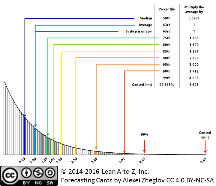
Finally, there are two quantitative shortcuts to estimating Weibull shape and scale parameters.

A good approximation of the scale parameter (thanks again to Troy for pointing this out) is the 63rd percentile. Indeed, the value of the Weibull cumulative distribution function where the random variable (lead time) equals the scale parameter is independent of the shape parameter and is given by:

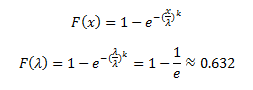
The value of the quantile (inverse cumulative distribution) function at this “magic point” is indeed the scale parameter as shown by:

The “magic point” has another important property, expressed by the following formula:

If the lead time data set is smooth enough to allow approximating the slope of the quantile function at the 63rd percentile (using, for example, finite differences), then this formula can be used to estimate the shape parameter.

Summary

• Weibull distribution occurs often in lead time data sets in creative industries. Estimating distribution parameters (shape and scale) is desirable so that we can use them in various quantitative models.
• The linear regression method is still preferable for finding the shape and scale parameters.
• In situations when the tools are not accessible, the shape and scale parameter can be approximated by comparison with several reference shapes. It is important to differentiate between three shape parameter ranges (k<1, 1<k<2, k>2) by observing convexity and concavity on the left side and the centre of the distribution curve.
• Relatively low precision (two-tenths for the shape parameters) is still sufficient for practical, quick thinking about the service delivery capability described by the lead time data set.
• There are two math tricks based on the unique properties of Weibull distribution and the 63rd percentile that can be used to roughly estimate the distribution parameters.