This post continues the series about lead-time distribution and deals with risks involved in matching real-world lead-time data sets to known distributions and estimating the distribution parameters.

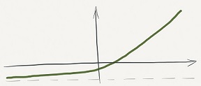
One of the key ideas of Nassim Nicholas Taleb’s book Antifragile is the notion of convexity, demonstrated by this option payoff curve. The horizontal axis shows the range of outcomes, the vertical axis shows the corresponding payoff. With this particular option, the payoff is asymmetric. Our losses in case of negative outcomes on the left are limited to a small amount. But our gains on the right side (positive outcomes) are unlimited. Note that this is due to the payoff function’s convexity. If the function was only increasing as a straight line, both our losses and gains would be unlimited.

A concave payoff function would achieve the opposite effect: limited gains and unlimited losses.

An antifragile system exposes itself to opportunities where benefits are convex and harm is concave and avoids exposure to the opposite.

In the book’s Appendix, Taleb considers a model that relies on Gaussian (normal) distribution. Suppose the Gaussian bell curve is centered on 0 and the standard deviation (sigma) is 1.5. What is the probability of the rare event that the random variable will exceed 6? It’s a number, and a pretty small one, which anyone with a scientific calculator can calculate.

Gaussian distribution analysis: probability of a rare event as a function of sigma is a convex function.

Right? Wrong. We don’t really know that sigma is 1.5. We simply calculated it from a set of numbers collected by observing some phenomenon. The real sigma may be a little bit more or a little bit less. How does that change the probability of our rare event? There is a chart in the Appendix, but I rechecked the calculations, and here it is — it’s a (very) convex function.

If we overestimate sigma a little bit, it’s really less than what we think it is, on the left side of the chart, we overestimate the probability of our rare event — a little bit. But if we underestimate sigma a little bit, we underestimate the probability of our rare event — a lot.

Convexity Effects in Lead Time Distributions

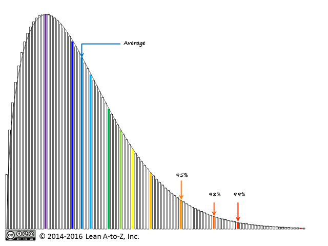
Weibull distribution analysis: probability of exceeding SLA as a function of parameter

Weibull distribution analysis: probability of exceeding SLA as a function of scale parameter (shape parameter k=3).

Let’s apply this convexity thinking to lead time distributions of service delivery in knowledge work. Weibull distributions with various parameters are often found in this domain. Let’s say we have a shape parameter k=1.5 and a service delivery expectation: 95% of deliveries within 30 days. If we are spot-on with our model, the probability to fail this expectation is exactly 5%. How sensitive is this probability to the shape and scale parameters?

With respect to the shape parameter, the probabilities to exceed the SLAs are all convex decreasing functions (I added the SLAs based on 98th and 99th percentiles to the chart). If we underestimate the shape parameter a bit, we overstate the risk a bit; if we overestimate it a bit, we understate the risk — a lot.

In other distribution shape types (k<1, k>2), it is the same story. The risk of underestimating-overestimating the shape parameter is asymmetric.

What about the scale parameter? It turns out there is less sensitivity with respect to it. The convexity effect (it pays to overestimate the scale parameter) is present for k>2 (as shown by the chart), it is weaker for 1<k<2, and the curves are essentially linear for k<1.

Conclusions

When analyzing lead time distributions of service delivery in creative industries, it is important not to overestimate the shape parameter. The under-overstatement of risk due to the shape parameter error is asymmetrical.

Matching a given lead-time data set to a distribution doesn’t have to be a complicated mathematical exercise. We should also not fool ourselves about the precision of this exercise, especially given our imperfect real-world data sets. Using several pre-calculated reference shapes should be sufficient for practical uses such as defining service level expectations, designing feedback loops and statistical process control. If we find our lead-time data set fits somewhere between two reference shapes, we should choose the smaller shape parameter.