I have introduced my forecasting cards and written about lead time distributions in my recent blog post series. Now I’d like to turn to how these concepts apply in iterative software development, particularly the popular process framework Scrum.

Let’s consider one of the reference distribution shapes (Weibull k=1.5), which often occurs in product development, particularly software. I went through various points on this curve and replaced them with what they ought to mean in this specific context.

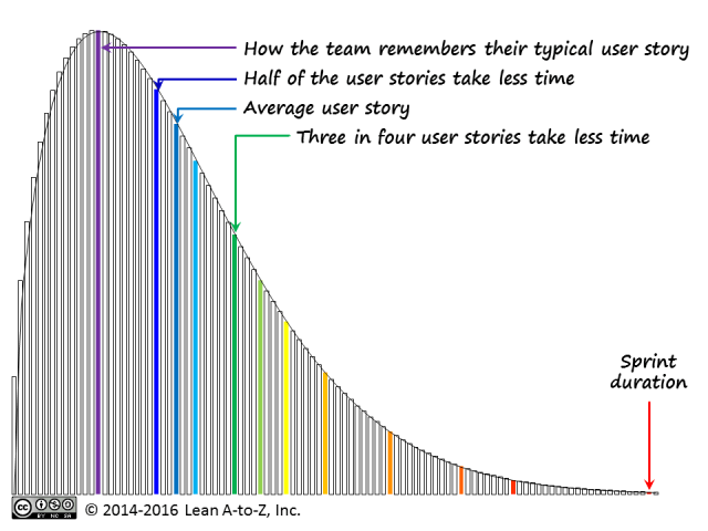
Scrum teams often complain that their user stories are not finished in the same sprint they were started. I have often observed in such situations that their stories are simply too large.

Even if typical stories were smaller than the duration of the sprint, such as, 7-8 days in a 10-business-day, two-week sprint, that was not small enough. The teams, Scrum masters, product owners held, perhaps subconsciously, the notion that we can “keep the average and squeeze the variance”, that is keep the 7-8-day average but limit variability — estimate, plan and task better — so that the right side of the distribution fits within the timebox. Recent lead time distribution research, examining many data sets from different companies (including those using iterative Agile methods) refute this notion. One of the key properties of common lead time distributions is that the average and standard deviation are not independent.

Another suggestion — keeping the average story to half the sprint duration, so that the ends of the bell curve gives us zero in the best case and the sprint duration in the worst case — is another illusion. Lead time distributions are asymmetric!

The real strategy is to left-shift the whole distribution curve.

This Kanban-sourced knowledge led to many quick wins as the Scrum teams, their Scrum masters and product owners I coached gave themselves a goal to systematically make their stories smaller. They simply asked, what can we do to double the count of delivered stories in the next few sprints, covering roughly the same workload in each sprint? After the doubling, ask the same question again until the stories are small enough.

How Small?

How small do user stories need to be? We can turn to our forecasting cards, which give the control-limit-to-average ratios between 3.9 and 4.9 for the two most common distribution shapes (1.25 and 1.5). In the extreme case, we have to assume the exponential distribution (I have observed quasi-exponential distributions in some cases in incremental software development), which gives us the ratio of 6.6. The ratio of average lead time to sprint duration in the range of 1:4 to 1:6 can be used as a guideline.

To make this rule of thumb a bit more practical, lets take into account these practical considerations: (1) the lead time is likely to be measured in whole days, (2) the number of business days in a sprint is likely to be a multiple of five, and (3) the median (half-longer, half-shorter) is easier to use in feedback loops than the average.

The control-limit-to-median ratios for the same distribution shapes are (consulting the forecasting cards again) 4.5 to 6.1; in the extreme case, 9.5. Therefore, half of the stories in one-fifth of the sprint duration can be used as a guideline. In the extreme cases, we may need one-tenth instead of one-fifth.

None of this is news to experienced Scrum practitioners, particularly those with eXtreme Programming backgrounds. XP tribe has appreciated the value of small stories since long ago, and invented and evangelized techniques, such as Product Sashimi to make them smaller.